Python: Images & pixels#
The goal of these sections is to provide an interactive illustration of image analysis concepts through the popular Python programming language.
Feel free to skip this!
If you’re more interested in concepts and/or ImageJ, I would recommend skipping the Python chapters at the beginning - you don’t need them to follow the rest of the book.
However, if you are interested, I hope these sections can help provide an alternative view of image analysis.
Even if you’ve never coded before, working through the examples will hopefully give you both a deeper understanding of image processing and some useful programming skills.
This page will introduce reading and displaying images. Later Python chapters in the handbook will build on these foundations.
Make it interactive!
Before continuing, you should make the notebook interactive so that you can run the code yourself - and explore what happens if you make changes.
Python overview
If you want a quick introduction to Python, check out the Python Primer section.
For lots more, see Robert Haase’s Bio-image Analysis Notebooks.
Read & show an image using Python #
Let’s begin by loading an image in Python, and then showing it using matplotlib.
"""
Read and display an image in Python.
"""
# In Python, we need to import things before we can use them
# (And, often, google to find out what we ought to be importing,
# then copy & paste the same import statements a lot)
import matplotlib.pyplot as plt
from imageio import imread
# Read an image - we need to know the full path to wherever it is
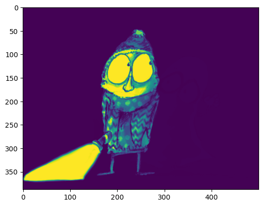
im = imread('../../../images/spooked.png')
# Create a plot of the image using the default brightness/contrast min/max and colormap
plt.imshow(im)
# Actually show the plot (if we don't do this explicitly, it might display anyway - but not always)
plt.show()
/tmp/ipykernel_3408/3771718922.py:12: DeprecationWarning: Starting with ImageIO v3 the behavior of this function will switch to that of iio.v3.imread. To keep the current behavior (and make this warning disappear) use `import imageio.v2 as imageio` or call `imageio.v2.imread` directly.
  im = imread('../../../images/spooked.png')
Changing lookup tables#
The key method here is plt.imshow.
We can pass additional parameters to customize the display in many ways.
To see what is possible, I usually start to type the name and then press Shift+Tab to prompt some documentation to appear.
plt.imshow(
Alternatively, you can run either of the following lines
?plt.imshow
help(plt.imshow)
to display some help text.
help(plt.imshow)
Help on function imshow in module matplotlib.pyplot:

imshow(X: 'ArrayLike | PIL.Image.Image', cmap: 'str | Colormap | None' = None, norm: 'str | Normalize | None' = None, *, aspect: "Literal['equal', 'auto'] | float | None" = None, interpolation: 'str | None' = None, alpha: 'float | ArrayLike | None' = None, vmin: 'float | None' = None, vmax: 'float | None' = None, origin: "Literal['upper', 'lower'] | None" = None, extent: 'tuple[float, float, float, float] | None' = None, interpolation_stage: "Literal['data', 'rgba'] | None" = None, filternorm: 'bool' = True, filterrad: 'float' = 4.0, resample: 'bool | None' = None, url: 'str | None' = None, data=None, **kwargs) -> 'AxesImage'
    Display data as an image, i.e., on a 2D regular raster.

    The input may either be actual RGB(A) data, or 2D scalar data, which
    will be rendered as a pseudocolor image. For displaying a grayscale
    image, set up the colormapping using the parameters
    ``cmap='gray', vmin=0, vmax=255``.

    The number of pixels used to render an image is set by the Axes size
    and the figure *dpi*. This can lead to aliasing artifacts when
    the image is resampled, because the displayed image size will usually
    not match the size of *X* (see
    :doc:`/gallery/images_contours_and_fields/image_antialiasing`).
    The resampling can be controlled via the *interpolation* parameter
    and/or :rc:`image.interpolation`.

    Parameters
    ----------
    X : array-like or PIL image
        The image data. Supported array shapes are:

        - (M, N): an image with scalar data. The values are mapped to
          colors using normalization and a colormap. See parameters *norm*,
          *cmap*, *vmin*, *vmax*.
        - (M, N, 3): an image with RGB values (0-1 float or 0-255 int).
        - (M, N, 4): an image with RGBA values (0-1 float or 0-255 int),
          i.e. including transparency.

        The first two dimensions (M, N) define the rows and columns of
        the image.

        Out-of-range RGB(A) values are clipped.

    cmap : str or `~matplotlib.colors.Colormap`, default: :rc:`image.cmap`
        The Colormap instance or registered colormap name used to map scalar data
        to colors.

        This parameter is ignored if *X* is RGB(A).

    norm : str or `~matplotlib.colors.Normalize`, optional
        The normalization method used to scale scalar data to the [0, 1] range
        before mapping to colors using *cmap*. By default, a linear scaling is
        used, mapping the lowest value to 0 and the highest to 1.

        If given, this can be one of the following:

        - An instance of `.Normalize` or one of its subclasses
          (see :ref:`colormapnorms`).
        - A scale name, i.e. one of "linear", "log", "symlog", "logit", etc.  For a
          list of available scales, call `matplotlib.scale.get_scale_names()`.
          In that case, a suitable `.Normalize` subclass is dynamically generated
          and instantiated.

        This parameter is ignored if *X* is RGB(A).

    vmin, vmax : float, optional
        When using scalar data and no explicit *norm*, *vmin* and *vmax* define
        the data range that the colormap covers. By default, the colormap covers
        the complete value range of the supplied data. It is an error to use
        *vmin*/*vmax* when a *norm* instance is given (but using a `str` *norm*
        name together with *vmin*/*vmax* is acceptable).

        This parameter is ignored if *X* is RGB(A).

    aspect : {'equal', 'auto'} or float or None, default: None
        The aspect ratio of the Axes.  This parameter is particularly
        relevant for images since it determines whether data pixels are
        square.

        This parameter is a shortcut for explicitly calling
        `.Axes.set_aspect`. See there for further details.

        - 'equal': Ensures an aspect ratio of 1. Pixels will be square
          (unless pixel sizes are explicitly made non-square in data
          coordinates using *extent*).
        - 'auto': The Axes is kept fixed and the aspect is adjusted so
          that the data fit in the Axes. In general, this will result in
          non-square pixels.

        Normally, None (the default) means to use :rc:`image.aspect`.  However, if
        the image uses a transform that does not contain the axes data transform,
        then None means to not modify the axes aspect at all (in that case, directly
        call `.Axes.set_aspect` if desired).

    interpolation : str, default: :rc:`image.interpolation`
        The interpolation method used.

        Supported values are 'none', 'antialiased', 'nearest', 'bilinear',
        'bicubic', 'spline16', 'spline36', 'hanning', 'hamming', 'hermite',
        'kaiser', 'quadric', 'catrom', 'gaussian', 'bessel', 'mitchell',
        'sinc', 'lanczos', 'blackman'.

        The data *X* is resampled to the pixel size of the image on the
        figure canvas, using the interpolation method to either up- or
        downsample the data.

        If *interpolation* is 'none', then for the ps, pdf, and svg
        backends no down- or upsampling occurs, and the image data is
        passed to the backend as a native image.  Note that different ps,
        pdf, and svg viewers may display these raw pixels differently. On
        other backends, 'none' is the same as 'nearest'.

        If *interpolation* is the default 'antialiased', then 'nearest'
        interpolation is used if the image is upsampled by more than a
        factor of three (i.e. the number of display pixels is at least
        three times the size of the data array).  If the upsampling rate is
        smaller than 3, or the image is downsampled, then 'hanning'
        interpolation is used to act as an anti-aliasing filter, unless the
        image happens to be upsampled by exactly a factor of two or one.

        See
        :doc:`/gallery/images_contours_and_fields/interpolation_methods`
        for an overview of the supported interpolation methods, and
        :doc:`/gallery/images_contours_and_fields/image_antialiasing` for
        a discussion of image antialiasing.

        Some interpolation methods require an additional radius parameter,
        which can be set by *filterrad*. Additionally, the antigrain image
        resize filter is controlled by the parameter *filternorm*.

    interpolation_stage : {'data', 'rgba'}, default: 'data'
        If 'data', interpolation
        is carried out on the data provided by the user.  If 'rgba', the
        interpolation is carried out after the colormapping has been
        applied (visual interpolation).

    alpha : float or array-like, optional
        The alpha blending value, between 0 (transparent) and 1 (opaque).
        If *alpha* is an array, the alpha blending values are applied pixel
        by pixel, and *alpha* must have the same shape as *X*.

    origin : {'upper', 'lower'}, default: :rc:`image.origin`
        Place the [0, 0] index of the array in the upper left or lower
        left corner of the Axes. The convention (the default) 'upper' is
        typically used for matrices and images.

        Note that the vertical axis points upward for 'lower'
        but downward for 'upper'.

        See the :ref:`imshow_extent` tutorial for
        examples and a more detailed description.

    extent : floats (left, right, bottom, top), optional
        The bounding box in data coordinates that the image will fill.
        These values may be unitful and match the units of the Axes.
        The image is stretched individually along x and y to fill the box.

        The default extent is determined by the following conditions.
        Pixels have unit size in data coordinates. Their centers are on
        integer coordinates, and their center coordinates range from 0 to
        columns-1 horizontally and from 0 to rows-1 vertically.

        Note that the direction of the vertical axis and thus the default
        values for top and bottom depend on *origin*:

        - For ``origin == 'upper'`` the default is
          ``(-0.5, numcols-0.5, numrows-0.5, -0.5)``.
        - For ``origin == 'lower'`` the default is
          ``(-0.5, numcols-0.5, -0.5, numrows-0.5)``.

        See the :ref:`imshow_extent` tutorial for
        examples and a more detailed description.

    filternorm : bool, default: True
        A parameter for the antigrain image resize filter (see the
        antigrain documentation).  If *filternorm* is set, the filter
        normalizes integer values and corrects the rounding errors. It
        doesn't do anything with the source floating point values, it
        corrects only integers according to the rule of 1.0 which means
        that any sum of pixel weights must be equal to 1.0.  So, the
        filter function must produce a graph of the proper shape.

    filterrad : float > 0, default: 4.0
        The filter radius for filters that have a radius parameter, i.e.
        when interpolation is one of: 'sinc', 'lanczos' or 'blackman'.

    resample : bool, default: :rc:`image.resample`
        When *True*, use a full resampling method.  When *False*, only
        resample when the output image is larger than the input image.

    url : str, optional
        Set the url of the created `.AxesImage`. See `.Artist.set_url`.

    Returns
    -------
    `~matplotlib.image.AxesImage`

    Other Parameters
    ----------------
    data : indexable object, optional
        If given, all parameters also accept a string ``s``, which is
        interpreted as ``data[s]`` (unless this raises an exception).

    **kwargs : `~matplotlib.artist.Artist` properties
        These parameters are passed on to the constructor of the
        `.AxesImage` artist.

    See Also
    --------
    matshow : Plot a matrix or an array as an image.

    Notes
    -----
    Unless *extent* is used, pixel centers will be located at integer
    coordinates. In other words: the origin will coincide with the center
    of pixel (0, 0).

    There are two common representations for RGB images with an alpha
    channel:

    -   Straight (unassociated) alpha: R, G, and B channels represent the
        color of the pixel, disregarding its opacity.
    -   Premultiplied (associated) alpha: R, G, and B channels represent
        the color of the pixel, adjusted for its opacity by multiplication.

    `~matplotlib.pyplot.imshow` expects RGB images adopting the straight
    (unassociated) alpha representation.
This can sometimes reveal an overwhelming amount of information, and it can take a bit of time to figure out how to identify the key bits.
The important plotting options for our purposes are
cmapto change the colormap (LUT)vminto change the pixel value corresponding to the first color in the colormapvmaxto change the pixel value corresponding to the last color in the colormap
The last two options control the brightness/contrast.
Try running the following code cells to see the effect, and try out other changes.
"""
Display an image with different brightness/contrast.
(Be sure to run the cells above before this one!)
"""

# Display the image with a grayscale colormap
plt.imshow(im, cmap='gray')
plt.show()

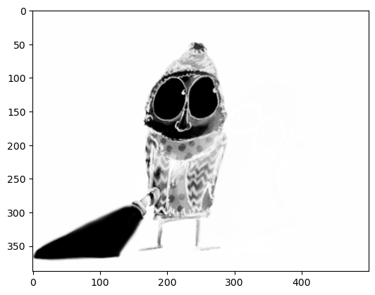
# Create an X-ray by adding '_r' to 'reverse' the colormap
plt.imshow(im, cmap='gray_r')
plt.show()
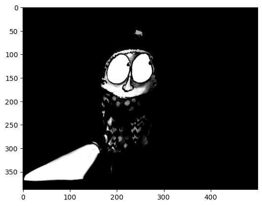
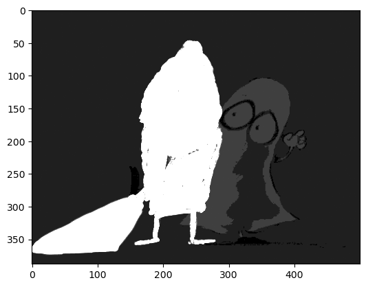
# Display the image with a grayscale colormap and modified brightness/contrast
plt.imshow(im, cmap='gray', vmin=100, vmax=255)
plt.show()
# Display the image with a grayscale colormap and modified brightness/contrast
plt.imshow(im, cmap='gray', vmin=0, vmax=8)
plt.show()
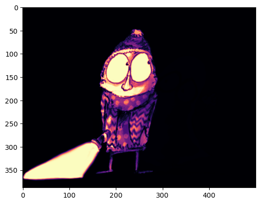
There are many more colormaps available in matplotlib – for details, see https://matplotlib.org/stable/tutorials/colors/colormaps.html
# Display with a 'perceptually uniform colormap'
plt.imshow(im, cmap='magma')
plt.show()
# Display with a colormap that is, frankly, not very helpful here
plt.imshow(im, cmap='hsv')
plt.show()
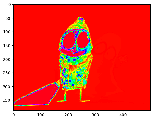
As you can see, the image may look very different depending upon the colormap and min/max values used.
However, it’s crucial that we haven’t modified the original image data itself.
To check this, try showing the image as we did initially - to make sure it looks the same.
# Display the image as before
plt.imshow(im)
plt.show()
Further customizing image display#
Lots more can be done to customize appearance.
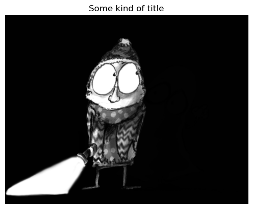
In order to standardize things throughout this book, I normally turn off the outer axis (numbers around the boundary), set an image title, and use a grayscale lookup table.
The code to do this is shown below.
# Load and display an image with a title & no visible axis
im = imread('../../../images/spooked.png')

plt.imshow(im, cmap='gray')
plt.axis(False)
plt.title('Some kind of title')
plt.show()
/tmp/ipykernel_3408/2843473488.py:2: DeprecationWarning: Starting with ImageIO v3 the behavior of this function will switch to that of iio.v3.imread. To keep the current behavior (and make this warning disappear) use `import imageio.v2 as imageio` or call `imageio.v2.imread` directly.
  im = imread('../../../images/spooked.png')
Writing functions#
If you use the same customizations frequently, it helps to define a function that applies them. Then you don’t need to copy and paste the same lines of code frequently; rather, you just call the function instead.
The function definition starts with
def. It is followed by
The function name
Parameters (within parentheses), sometimes with default values
A colon
The main code that implements the function - this needs to be indented (something Python is very fussy about)
def my_imshow(im, title=None, cmap='gray'):
"""
Call imshow and turn the axis off, optionally setting a title and colormap.
The default colormap is 'gray', and there is no default title.
"""
# Show image & turn off axis
plt.imshow(im, cmap=cmap)
plt.axis(False)
# Show a title if we have one
if title is not None:
plt.title(title)
plt.show()
# Now I just need to call my function rather than customize every plot
my_imshow(im, title='Here is my new title')
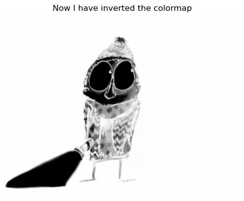
my_imshow(im, title='Now I have inverted the colormap', cmap='gray_r')

Helper functions in this book#
I’ve written several helper functions to standardize image display throughout this handbook. They aren’t part of any wider Python library, but we can use them here to make our scripts shorter and focus on the more important concepts.
To use these helper functions, we need to import them once per Jupyter notebook.
Then we can use the methods such as load_image and show_image (along with companions like show_histogram) to display images.
# Default imports (they are already included at the top of the page)
import sys
sys.path.append('../../../')
from helpers import *
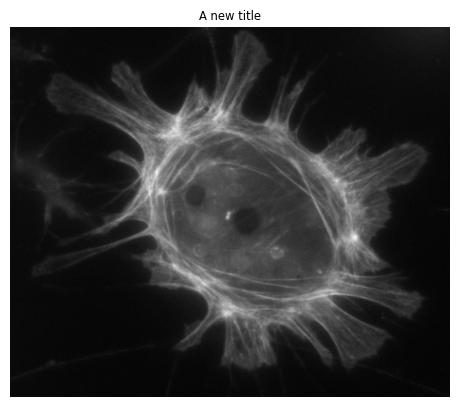
# Easier way to load and display an image, which we'll use from now on
im = load_image('sunny_cell.tif')
show_image(im, title='A new title')