ImageJ: Filters

Show code cell content Hide code cell content

%load_ext autoreload
%autoreload 2

# Default imports
import sys
sys.path.append('../../../')
from helpers import *
from matplotlib import pyplot as plt
from myst_nb import glue
import numpy as np
from scipy import ndimage

Introduction

Most of the filters we’ve considered are available through the Process ‣ Filters submenu. This section adds a little more information about their implementation in ImageJ, and asks a few questions.

Linear filters

Mean filters

The easiest way to apply a 3×3 mean filter in ImageJ is through the Process ‣ Smooth command. The fact that the shortcut is Shift+S can almost make this too easy, as I find myself accidentally smoothing when I really wanted to save my image. Take care.

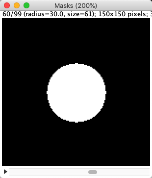
To apply larger mean filters, the command is Process ‣ Filters ‣ Mean…. It uses approximately circular neighborhoods, and the neighborhood size is adjusted by choosing a Radius value. The Process ‣ Filters ‣ Show Circular Masks command displays the neighborhoods used for different values of Radius. If you happen to choose Radius = 1, you get a 3×3 filter – and the same results as using Smooth.

Gaussian filters

Process ‣ Filters ‣ Gaussian Blur… is the command that implements a Gaussian filter.

In the event that you want a Gaussian filter that isn’t isotropic (i.e. has a different size along different dimensions), Process ‣ Filters ‣ Gaussian Blur 3D… can be used.

Although not really recommended, unsharp masking is available through Process ‣ Filters ‣ Unsharp mask….

Difference of Gaussians

There’s currently no direct command in ImageJ to implement difference of Gaussians filtering, rather the steps need to be pieced together with image duplication and subtraction. However Difference of Gaussians describes how to generate a macro for DoG filtering.

Custom linear filters

Process ‣ Filters ‣ Convolve… makes it possible to define any custom linear filter by entering the values of the desired coefficients, separated by spaces and arranged in rows and columns. If you Normalize Kernel is selected, then the coefficients are scaled so that they add to 1, by dividing by the sum of all the coefficients – unless the sum is 0, in which case requesting normalizion does nothing.

Question

When defining an n_×_n filter kernel with Convolve…, ImageJ insists that n is an odd number. Why?

Answer

If n is an odd number, the filter has a clear central pixel. This makes it possible to center the filter kernel on a pixel on the image.

Question

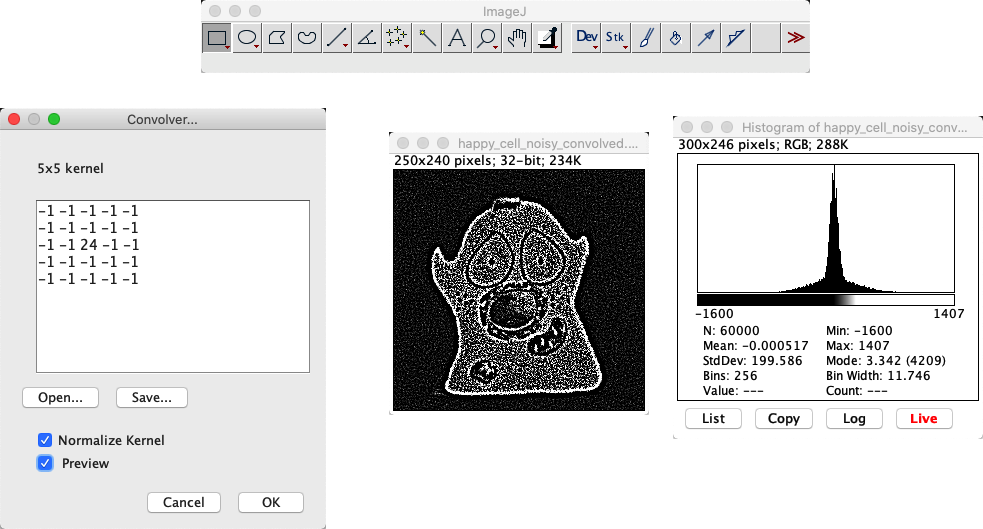
Predict what happens when you convolve an image using a filter that consists of a single coefficient with a value -1 in the following cases:

1. Normalize Kernel is checked

2. You have a 32-bit image, Normalize Kernel is unchecked

3. You have an 8-bit image, Normalize Kernel is unchecked

Answer

The results of convolving with a single -1 coefficient in different circumstances:

1. Normalize Kernel is checked: Nothing at all happens. The normalization makes the filter just a single 1… and convolving with a single 1 leaves the image unchanged.

2. You have a 32-bit image (Normalize Kernel unchecked): The pixel values become negative, and the image looks inverted.

3. You have an 8-bit image (Normalize Kernel unchecked): The pixel values would become negative, but then cannot be stored in an 8-bit unsigned integer form. Therefore, all pixels simply become clipped to zero.

Practical

Using any image, work out which of the methods for dealing with boundaries shown in Fig. 86 is used by ImageJ’s Convolve… command.

Note: This requires a bit of creativity. It will certainly help to use an image with some variation at the image boundary. I used File ‣ Open Samples ‣ Blobs.

Solution

Replication of boundary pixels is the default method used by Process ‣ Filters ‣ Convolve… in ImageJ (although other filtering plugins by different authors might use different methods).

My approach to test this involved using Convolve… with a filter that consisting of a 1 followed by a lot of zeros (e.g. 1 0 0 0 0 0 0 0 0 0 0 0 0...). This basically shifts the image to the right, bringing whatever is outside the image boundary into view.

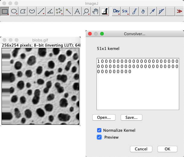
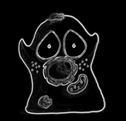
Fig. 100 Gradient magnitude

Practical

Practice using the commands we’ve met so far by determining the gradient magnitude of an image, as described here.

You will need to use

• Image ‣ Duplicate…

• Process ‣ Filters ‣ Convolve…

• Process ‣ Image Calculator…

• Several commands in the Process ‣ Math submenu

• Something else we’ve used before… possibly

If you need a sample image, you can use File ‣ Open samples ‣ Blobs (25K). (Be sure to pay attention to the bit-depth!)

Solution

The process to calculate the gradient magnitude is:

1. Convert the image to 32-bit (if it isn’t already 32-bit)

2. Duplicate the image

3. Convolve one copy of the image with the horizontal gradient filter, and one with the vertical (i.e. coefficients -1 0 1 arranged as a row or column)

4. Compute the square of both images (Process ‣ Math ‣ Square)

5. Use the image calculator to add the images together

6. Compute the square root of the resulting image (Process ‣ Math ‣ Square Root)

Here’s a macro that implements these steps:

run("32-bit");

id1 = getImageID()
run("Duplicate...", " ");
id2 = getImageID();

run("Convolve...", "text1=[-1 0 1\n] normalize");
run("Square");

selectImage(id1);
run("Convolve...", "text1=-1\n0\n1\n normalize");
run("Square");

imageCalculator("Add create", id1, id2);
run("Square Root");

The convolution results in negative values, which is why the 32-bit conversion is needed.

Note: This is (almost) what is done by the command Process ‣ Find Edges, except the gradient filters are slightly different.

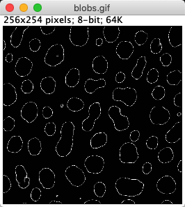
Fig. 101 The ‘Edges’ LUT

Practical

ImageJ has a LUT called edges under Image ‣ Lookup Tables ‣ Edges. Applied to File ‣ Open samples ‣ Blobs (25K), it does a rather good job of highlighting edges – without actually changing the pixels at all.

How does it work? Does it apply a filter?

Solution

The edges LUT shows most low and high pixel values as black – and uses lighter shades of gray only for a small range of values in between (see Image ‣ Color ‣ Edit LUT…). In any image with a good separation of background and foreground pixels, but which still has a somewhat smooth transition between them, this means everything but the edges can appear black.

All this is achieved by a LUT: no pixels were harmed, there was no filtering applied.

Nonlinear filters

Rank filters

The main rank filters are to be found exactly where you might expect them:

• Process ‣ Filters ‣ Median…

• Process ‣ Filters ‣ Minimum…

• Process ‣ Filters ‣ Maximum…

ImageJ uses circular neighborhoods with its built-in rank filters, similar to how mean filters are implemented. We will meet these filters again in Morphological operations.

Removing outliers

Fig. 88 shows that median filtering is much better than mean filtering for removing outliers. We might encounter this if something in the microscope is not quite functioning as expected or if dark noise is a problem, but otherwise we expect the noise in fluorescence microscopy images to produce few really extreme values (see Noise).

Nevertheless, Process ‣ Noise ‣ Remove Outliers… provides an alternative if isolated bright values are present. This is a nonlinear filter that inserts median values only whenever a pixel is found that is further away from the local median than some adjustable threshold.

It’s therefore like a more selective median filter that will only modify the image at pixels where it is considered really necessary.