ImageJ: Pixel size & dimensions#
Introduction#
This section will explore pixel sizes and dimensions in ImageJ. Along the way, we will see how to generate scale bars and fix images where the pixel size or dimensions are incorrect – at least whenever we know what the correct values are.
Pixel sizes & Properties#
You can see the pixel size for an image in ImageJ under . These are provided separately as values for Pixel width and Pixel height.
There is also an additional value, Voxel depth, which is only relevant for z-stacks; this gives the spacing between z-slices.
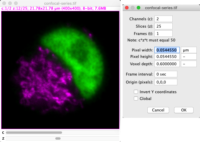
Fig. 43 Image properties for the Confocal Series sample, which include the pixel size.#
If the pixel size information is unavailable, the pixel sizes are given as 1 pixel: not terribly informative. Otherwise, the pixel sizes are given in the units displayed nearby in the properties dialog.
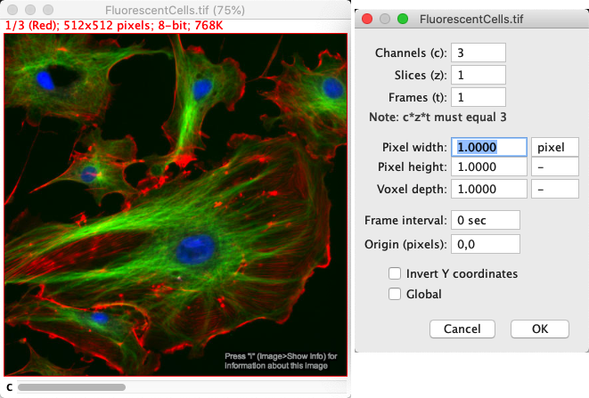
Fig. 44 Image properties for the Fluorescent Cells sample, which do not include useful pixel size information.#
The pixel width and height are usually the same. The voxel depth (where relevant) is often different.
One way to check if the pixel size information is set for an image is to use
How else can you check this, even more easily?
Tip: The answer should already be visible in Fig. 43 and Fig. 44.
The size of the image is given at the top of each image window. If the pixel size information is available, this is given in calibrated units. Otherwise, it is given only in pixels.
Pixel sizes & measurements#
As described before, the pixel size influences measurements in ImageJ – but the units don’t appear anywhere in the Results table. Furthermore, once a measurement is added to the Results table it is fixed: it won’t automatically update if the pixel sizes are changed later.
For that reason, you need to be careful to check pixel sizes before making any measurements and make sure it’s clear to you which units have been used.
Fig. 45 The same ROI (here, a 100 x 100 pixel square) can appear to have a different area if it is measured on images that have different pixel sizes. The measurement is converted before being added to the Results table, but the units are not included.#
Setting the pixel size#
If the pixel size information is missing, but you know what it should be, you can simply enter the required width and height values in the Properties… dialog box.
Typing µm
Depending upon your computer, typing µm for the units might be tricky. Fortunately, typing um works as well – ImageJ automatically converts um → µm.
If you don’t know what the pixel size should be, but you do know the length of some structure in your image, then you can
Draw a line along the known structure with the line tool

Run .
This will automatically populate the Distance in pixels based upon the length of the line. You can then input the known physical length and units, then click OK. You should check to confirm that the values have been updated sensibly.
Fig. 46 Setting the pixel size in an image by inserting the length of a known structure.#
Using Set Scale…
Ideally, would be used with a calibration slide to establish the pixel sizes reliably. The values can then be transferred to other images acquired with the same settings using (or a macro).
Beware that, if you have drawn a line as described above, the Distance in pixels value is initialized from that line – so don’t change that. Rather, do change the Known distance and Unit of length values according to the physical length indicated by the line.
If the Unit of length should be µm but your keyboard lacks a µ, you can type um instead.
Showing a scale bar#
It’s generally good practice to include a scalebar in any figures. This is only really meaningful if the pixel sizes are set correctly within the image properties.
You can create a scalebar using .
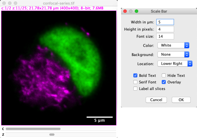
Fig. 47 Setting a scale bar as an overlay.#
There are several options that can be used to adjust the appearance of the scalebar. One of the most important is the Overlay option, because this determines whether the scalebar is ‘burned in’ to the image (i.e. the pixel values are modified) or if it’s instead added as a (text) ROI as part of the image overlay.
My advice is to always add the scalebar as an overlay. That means you can remove it again, or adjust its appearance. The only disadvantage is that, if you save the image immediately, it might not appear in other software. The solution is to generate an RGB image that includes the overlay as a final step before saving, by using .
Stacks & Hyperstacks#
2D images have been around since the beginning. Then ImageJ supported stacks, which allowed an extra dimension that could either include different time points or z-slices – but not both. Nowadays, hyperstacks are the more flexible derivative of stacks, and can (currently) store up to 5 dimensions without getting them confused.
Hyperstack flexibility
A hyperstack can contain 0–5 dimensions, while a stack can only contain 0–3. So why worry about stacks at all?
The main reason comes from ImageJ’s evolution over time. Some commands – perhaps originating in the pre-hyperstack era -– were written only for 2D or 3D data. Trying to apply them to 4D or 5D images may then cause an error, or it may simply produce strange results.
In practice, this is unlikely to be an issue nowadays. Hyperstacks have been around for so long now that all major commands that work on stacks should also handle hyperstacks properly. Nevertheless, it helps to have a historical perspective to understand why both terms still exist in ImageJ’s interface.
It may also help if you encounter some very old plugin that was written for stacks but that doesn’t handle hyperstacks properly.
Navigating dimensions#
With a stack or hyperstack, only a single 2D slice is ‘active’ at any one time. A (hyper)stack image window can have up to 3 sliders, used to navigate the channels, z and time dimensions and select the active slice. In the case of multichannel images (where there is a ‘channel’ dimension), any changes to lookup tables are made for all the slices on the currently-active channel.

Fig. 48 A 5D image viewed in ImageJ.#
Correcting dimensions#
Like the pixel size, the dimensions of an image can found under .
Sometimes the dimensions can be incorrect. This might happen, for example, if different z-slices were wrongly interpreted as time points when a file was opened, or the presence of multiple channels was not spotted. Misinterpreting the dimensions can not only affect the display of the image, but also some processing and measurements.
It’s also possible to change the dimensions through , but I find that can sometimes be unreliable because of the old stack/hyperstack distinction (i.e. it doesn’t convert a stack to a hyperstack, and therefore doesn’t display all the sliders that are needed). A better option is to use to fix dimensions.
Something terrible has befallen the file lost_dimensions.tif, so that it’s displayed as a 3D stack, when in reality it should have more dimensions.
By inspecting the file, identify how many channels, z-slices and time points it originally contained, and set these using so that it displays properly. What are the correct dimensions?
![]()
lost_dimensions.tif should contain 2 channels, 3 z-slices and 16 time points.
The dimensions are in the default order (xyczt).
Plots and profiles#
More dimensions can make data harder to visualize and interpret. Reducing dimensions can help.
can be used to generate a 1D plot of pixel values along a line within the image.
To use it, you can first draw a line ROI .
By default, pixel values occurring along the line will be displayed in the plot, however it’s possible to average multiple pixels perpendicular to line if needed.
To do this, double-click on the line tool and adjust the Line width value.
It’s also possible to apply K to a rectangle  , in which case it will average pixels vertically (default) or horizontally (if the Alt key is pressed).
Another option if you have a stack or hyperstack is to use to generate a profile across the slices. This essentially plots the mean value within any ROI (or across the whole image) for every slice in the stack. Perhaps unexpectedly, the same command is able to generate a profile across time points as well; when necessary, a dialog is shown to choose the dimension.
In all cases, profile plots contain a Live button. This means the plot data updates as any changes are made to the image, including ROIs being generated and moved around.
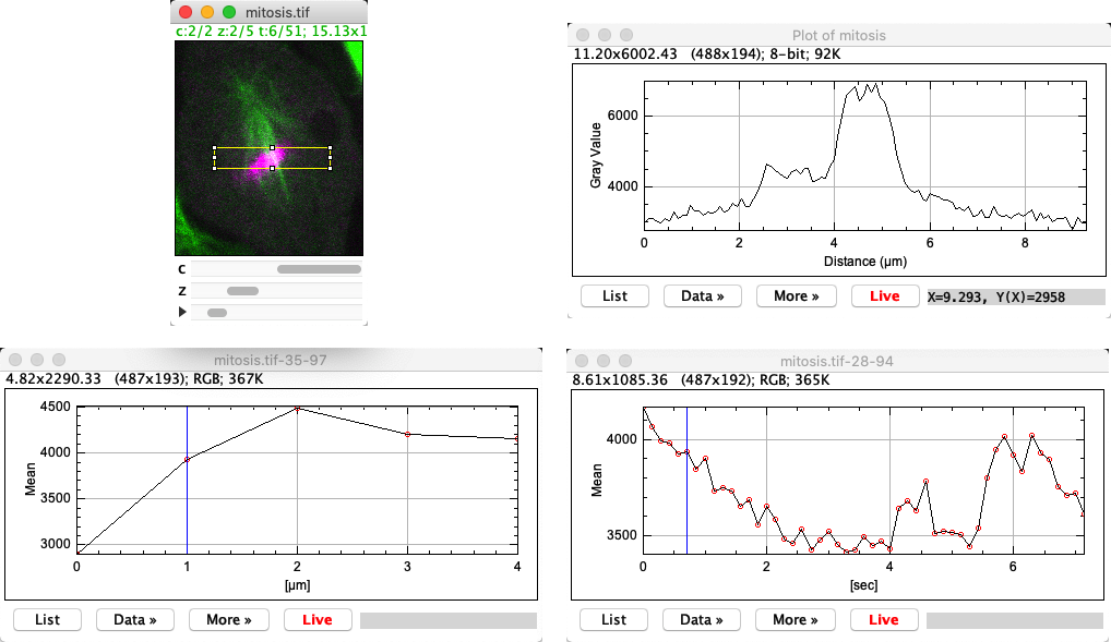
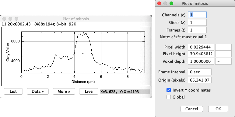
Fig. 49 Three different profile plots, based on a rectangle. (Top) A regular profile plot from the active 2D slice, using . (Bottom) Profiles generated by along the z-axis (left) and across time points (right).#
Create a profile plot from any image, by drawing a line ROI and pressing K.
As far as ImageJ is concerned, the profile plot itself is an image – albeit a strange one. This means you can use to check the pixel size of the profile plot.
What do you notice about the pixel sizes?
![]()
You will probably see that the pixel width and height are different. In fact, the pixel width depends upon the scaling of the x-axis and the pixel height depends upon the scaling of the y-axis.
This can be quite useful, because it means you can make measurements within the profile plot itself.
If you want to measure a distance along the x or y axis, you can use the line tool while pressing Shift.
This forces the line to be perfectly horizontal or perfectly vertical; without Shift it would be easy to draw a line at a slight diagonal that could give incorrect results.
Displaying dimensions#
Z-projections#
The command to generate a z-projection in ImageJ is . This supports several different projection types, as shown in Fig. 50.
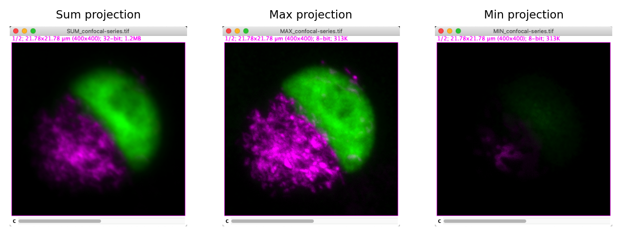
Fig. 50 Three projections of a z-stack. Sum projections often look similar to maximum projections, but less sharp.#
Imagine computing a sum and a maximum projection of a 10-slice stack containing a large, in-focus nucleus. How might each of these projections be affected if your stack contained:
4 additional, out-of-focus slices (with non-zero pixel values)
several very bright, isolated, randomly distributed outlier pixels – with values twice what they should be (due to noise)
Additional, out-of-focus planes will have an effect upon sum projections: increasing all the resulting pixel values. However, the extra planes would have minimal effects upon maximum projections, since they are unlikely to contain higher values than the in-focus planes.
Maximum projections will, however, be very affected by bright outliers: these will almost certainly appear in the result with their values unchanged. Such outliers would also influence a sum projection, but less drastically because each pixel would contain the sum of 9 reasonable values and only 1 large value (unless, by bad luck or a dubious detector, many outliers happen to overlap at the same xy coordinate).
What happens if you calculate a maximum projection twice for the 5D image ?
By this I mean you run on the original image, and then again on the output of the first projection.
![]()
You should end up with a maximum z-projecton followed by a time projection!
If there is a time dimension but no z dimension, will use time instead.
If there is a z dimension but you want a time projection anyway, you could try careful use of or to temporarily switch the dimension names and trick ImageJ into doing what you want.
Orthogonal views#
The command makes it possible to generate interactive orthogonal slices from an image stack. This opens up 2 extra windows, so that when you click at any point on the original xy view, you are shown cross-sections through that point from each direction.
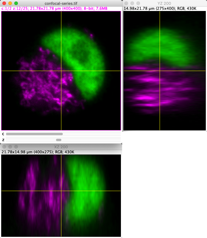
Fig. 51 Orthogonal views in ImageJ.#
Note that when viewing the orthogonal slices, clicks on the image are intercepted. This makes it difficult to interact with the image normally or create new ROIs. If you close any of the additional views then the command is deactivated, and you can go back to working with the image as before.
Reslicing#
If you look closely at the orthogonal slices, you will see that they are RGB images – even if the original stack is not RGB. They are also locked to using the LUT and brightness/contrast settings that were active when the command was first run.
This makes them a useful visualization trick, but they do not provide a rotated version of the data for analysis.
If you instead want to rotate the entire stack so that you can browse through what are effectively xz or yz slices and do whatever you want to them, the command you need is .
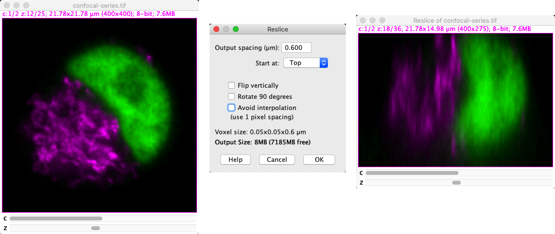
Fig. 52 Reslicing an image.#
After reslicing, you can then use to effectively generate orthogonal z-projections.
Reslicing and interpolation
Interpolation effectively means making up plausible new pixel values to fill in the gaps ‘between’ known pixels. In this case, interpolation handles the fact that the pixel width, pixel height and voxel depth (z-spacing) are seldom identical.
With that in mind, if you need to reslice an image then I recommend trying it both with and without Avoid pixel interpolation selected, checking the pixel size under in both cases. Seeing what actually happens is likely to be more informative than trying to make sense of any explanation I could try to give.