Simulating image formation#
Introduction#
The Difference of Gaussians macro developed in ImageJ: Writing macros was useful, but quite simple. This section contains an extended practical, the goal of which is to develop a somewhat more sophisticated macro that takes an ‘ideal’ image, and then simulates how it would look after being recorded by a fluorescence microscope. It can be used not only to get a better understanding of the image formation process, but also to generate test data for analysis algorithms. By creating simulations with different settings, we can investigate how our results might be affected by changes in image acquisition and quality.
Image formation summary#
The following is a summary of the aspects of image formation discussed in this book:
Images are composed of pixels, each of which has a single numeric value (not a color!).
The value of a pixel in fluorescence microscopy relates to a number of detected photons – or, more technically, the charge of the electrons produced by the photons striking a detector.
Images can have many dimensions. The number of dimensions is essentially the number of things you need to know to identify each pixel (e.g. time point, channel number, x coordinate, y coordinate, z slice).
The two main factors that limit image quality are blur and noise. Both are inevitable, and neither can be completely overcome.
Blur is characterized by the point spread function (PSF) of the microscope, which is the 3D volume that would be the result of imaging a single light-emitting point. It acts as a convolution.
In the focal plane, the image of a point is an Airy pattern. Most of the light is contained within a central region, the Airy disk.
The spatial resolution is a measure of the separation that must exist between structures before they can adequately be distinguished as separate, and relates to the size of the PSF (or Airy disk in 2D).
The two main types of noise are photon noise and read noise. The former is caused by the randomness of photon emission, while the latter arises from imprecisions in quantifying numbers of detected photons.
Detecting more photons helps to overcome the problems caused by both types of noise.
Different types of microscope have different advantages and costs in terms of spatial information, temporal resolution and noise.
PMTs are used to detect photons for single pixels, while CCDs and EMCCDs are used to detect photons for many pixels in parallel.
The macro in this chapter will work for 2D images, and simulate the three main components:
the blur of the PSF
photon noise
read noise
Furthermore, the macro will ultimately be written in such a way that allows us to investigate the effects of changing some additional parameters:
the size of the PSF (related to the objective lens NA and microscope type)
the amount of fluorescence being emitted from the brightest region
the amount of background (from stray light and other sources)
the exposure time (and therefore number of detected photons)
the detector’s offset
the detector’s gain
the detector’s read noise
camera binning
bit-depth
Recording the main steps#
It doesn’t really matter which image you use for this, but I recommend a single-channel 2D image that starts out without any obvious noise (e.g. the Happy cell.tif image). After starting the macro recorder, complete the following steps to create the main structure for the macro:
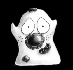
Fig. 163 Example input image#
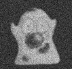
Fig. 164 Example output image#
Ensure the starting image is 32-bit.
Run using a sigma value of 2 to simulate the convolution with the PSF.
Here, we will assume that there are some background photons from other sources, but around the same number at every pixel in the image. So we can simply add a constant to this image using . The value should be small, perhaps 10.
The image now contains the ‘average rates of photon emission’ that we would normally like to have for one particular exposure time (i.e. it is noise-free). If we change the exposure time, we should change the pixel values similarly so that the rates remain the same. Because adjusting the exposure works like a multiplication, we can use the command. Set it to a ‘default’ value of 1 for now.
To convert the photon emission rates into actual photon counts that we could potentially detect, we need to simulate photon noise by replacing each pixel by a random value from a Poisson distribution that that has the same \(\lambda\) as the rate itself. At the time of writing, there’s no built-in command in ImageJ or Fiji to simulate Poisson noise but we can install RandomJ using the instructions at https://imagescience.org/meijering/software/randomj/. Then add noise by calling , making sure to set the Insertion: value to Modulatory. The Mean value will be ignored, so its setting does not matter.
Notice that all the pixels should now have integer values: you cannot detect parts of photons.
The detector gain scales up the number of electrons produced by detected photons. Make room for it by including another multiplication, although for now set the value to 1 (i.e. no extra gain).
Simulate the detector offset by adding another constant, e.g. 100.
Add read noise with , setting the standard deviation to 5.
Clip any negative values, by running and setting the value to 0.
Clip any positive values that exceed the bit-depth, by running . To assume an a 8-bit image, set the value to 255.
Now is a good time to clean up the code by removing any unnecessary lines, adding suitable comments, and bringing any interesting variables up to the top of the macro so that they can be easily modified later (as in Difference of Gaussians). We should also duplicate the image to avoid accidentally modifying the original. The end result should look something like this:
// Variables to change
psfSigma = 2;
backgroundPhotons = 10;
exposureTime = 1;
readStdDev = 5;
detectorGain = 1;
detectorOffset = 100;
maxVal = 255;

// Duplicate the image, to avoid changing the original
// Including " " means the default name will be used &
// we don't need to specify any other
run("Duplicate...", " ");

// Retain a reference so we can close the duplicate at the end
// (since RandomJ Poisson creates another new window)
idTemp = getImageID();

// Ensure image is 32-bit
run("32-bit");

// Simulate PSF blurring
run("Gaussian Blur...", "sigma="+psfSigma);

// Add background photons
run("Add...", "value="+backgroundPhotons);

// Multiply by the exposure time
run("Multiply...", "value="+exposureTime);

// Simulate photon noise
run("RandomJ Poisson", "mean=1.0 insertion=modulatory");

// Simulate the detector gain
run("Multiply...", "value="+detectorGain);

// Simulate the detector offset
run("Add...", "value="+detectorOffset);

// Simulate read noise
run("Add Specified Noise...", "standard="+readStdDev);

// Clip any negative values
run("Min...", "value=0");

// Clip the maximum values based on the bit-depth
un("Max...", "value="+maxVal);
You would have a perfectly respectable macro if you stopped now, but the following section contains some ways in which it may be improved.
Making improvements#
Normalizing the image#
The results you get from running the above macro will change depending upon the original range of the image that you use: that is, an image that starts off with high-valued pixels will end up having much less noise. To compensate for this somewhat, we can first normalize the image so that all pixels fall into the range 0–1. To do this, we need to determine the current range of pixel values, which can be found out using the macro function:
getStatistics(area, mean, min, max);
After running this, four variables are created giving the mean,
minimum and maximum pixel values in the image, along with the total image area.
Normalization is now possible using and commands, and adjusting their values. In the end this gives us
getStatistics(area, mean, min, max);
run("Subtract...", "value="+min);
divisor = max - min;
run("Divide...", "value="+divisor);
Varying the fluorescence emission rate#
The new problem we will have after normalization is that there will be a maximum photon emission rate of 1 in the brightest part of the image, which will give us a image dominated completely by noise. We can change this by multiplying the pixels again, and so define what we want the emission rate to be in the brightest part of the image. I suggest creating a variable for this, and setting its value to 10. Then add the following line immediately after normalization:
run("Multiply...", "value="+maxPhotonEmission);
Modifying this value allows you to change between simulating samples that are fluorescing more or less brightly. For a less bright sample, you will most likely need to increase the exposure time to get a similar amount of signal – but beware that increasing the exposure time also involves collecting more unhelpful background photons, so is not quite so good as having a sample where the important parts are intrinsically brighter.
Simulating binning#
The main idea of binning is that the electrons from multiple pixels are added together prior to readout, so that the number of electrons being quantified is bigger relative to the read noise. For 2×2 binning this involves splitting the image into distinct 2×2 pixel blocks, and creating another image in which the value of each pixel is the sum of the values within the corresponding block.
This could be done using the command, with a shrink factor of 2 and the Sum bin method. The macro recorder can again be used to get the main code that is needed. After some modification, this becomes
 if (doBinning) {
   run("Bin...", "x=2 y=2 bin=Sum");
 }
By enclosing the line within a code block (limit by the curly brackets) and beginning the block with if (doBinning), it’s easy to control whether binning is applied or not.
You simply add an extra variable to your list at the start of the macro
doBinning = true;
to turn binning on, or
doBinning = false;
to turn it off. The lines of code that perform the binning should be inserted before the addition of read noise.
Varying bit-depths#
Varying the simulated bit-depths by changing the maximum value allowed in the image takes a little work: you need to know that the maximum value in an 8-bit image is 255, while for a 12-bit image it is 4095 and so on.
It is more intuitive to just change the image bit-depth and have the macro do the calculation for you.
To do this, you can replace the maxVal = 255; variable at the start of the macro with nBits = 8; and then update the later clipping code to become
maxVal = pow(2, nBits) - 1;
run("Max...", "value="+maxVal);
Here, pow(2, nBits) is a function that gives you the value of 2nBits.
Now it’s easier to explore the difference between 8-bit, 12-bit and 14-bit images (which are the main bit-depths normally associated with microscope detectors, even if the resulting image is stored as 16-bit).
Rounding to integer values#
The macro has already clipped the image to a specified bit-depth, but it still contains 32-bit data and so potentially has non-integer values that could not be stored in the 8 or 16-bit images a microscope typically provides as output. Therefore it remains to round the values to the nearest integer.
There are a few ways to do this: we can convert the image using commands, though then we need to be careful about whether there will be any scaling applied. However, we can avoid thinking about this if we just apply the rounding ourselves. To do it we need to visit each pixel, extract its value, round the value to the nearest whole number, and put it back in the image. This requires using loops. The code, which should be added at the end of the macro, looks like this:
// Get the image dimensions
width = getWidth();
height = getHeight();

// Loop through all the rows of pixels
for (y = 0; y < height; y++) { // Loop through all the columns of pixels
  for (x = 0; x < width; x++) { // Extract the pixel value at coordinate (x, y)
    value = getPixel(x, y); // Round the pixel value to the nearest integer
    value = round(value); // Replace the pixel value in the image
    setPixel(x, y, value);
  }
}
This creates two variables, x and y, which are used to store the horizontal and vertical coordinates of a pixel.
Each starts off set to 0 (so we begin with the pixel at 0,0, i.e.
in the top left of the image). The code in the middle is run to set the first pixel value, then the variable x is incremented to become 1 – because x++ means add 1 to x.
This process is repeated so long as x is less than the image width, x < width.
When x eventually becomes equal to the width, it means that all pixel values on the first row of the image have been rounded.
Then y is incremented and x is reset to zero, before the process repeats and the next row is rounded as well.
This continues until y is equal to the image height – at which point the processing is complete [1].
Final code#
The final code of my version of the macro is given below:
// Variables to change
psfSigma = 2;
backgroundPhotons = 10;
exposureTime = 10;
readStdDev = 5;
detectorGain = 1;
detectorOffset = 100;
nBits = 8;
maxPhotonEmission = 10;
doBinning = false;

// Duplicate the image, to avoid changing the original
// Including " " means the default name will be used &
// we don't need to specify any other
run("Duplicate...", " ");

// Retain a reference so we can close the duplicate at the end
// (since RandomJ Poisson creates another new window)
idTemp = getImageID();

// Ensure image is 32-bit
run("32-bit");

// Normalize the image to the range 0-1
getStatistics(area, mean, min, max);
run("Subtract...", "value="+min);
divisor = max - min;
run("Divide...", "value="+divisor);

// Define the photon emission at the brightest point
run("Multiply...", "value="+maxPhotonEmission);

// Simulate PSF blurring
run("Gaussian Blur...", "sigma="+psfSigma);

// Add background photons
run("Add...", "value="+backgroundPhotons);

// Multiply by the exposure time
run("Multiply...", "value="+exposureTime);

// Simulate photon noise
run("RandomJ Poisson", "mean=1.0 insertion=modulatory");

// Simulate the detector gain
// (note this should really add Poisson noise too!)
run("Multiply...", "value="+detectorGain);

// Simulate binning (optional)
if (doBinning) {
 run("Bin...", "x=2 y=2 bin=Sum");
}

// Simulate the detector offset
run("Add...", "value="+detectorOffset);

// Simulate read noise
run("Add Specified Noise...", "standard="+readStdDev);

// Clip any negative values
run("Min...", "value=0");

// Clip the maximum values based on the bit-depth
maxVal = pow(2, nBits) - 1;
run("Max...", "value="+maxVal);

// Get the image dimensions
width = getWidth();
height = getHeight();

// Round the pixels to integer values
for (y = 0; y < height; y++) {
   // Loop through all the columns of pixels
   for (x = 0; x < width; x++) {
       // Extract the pixel value at coordinate (x, y)
       value = getPixel(x, y);
       // Round the pixel value to the nearest integer
       value = round(value);
       // Replace the pixel value in the image
       setPixel(x, y, value);
   }
}

// Reset the display range (i.e. image contrast)
resetMinAndMax();

// Close the temporary image
selectImage(idTemp);
close();
Uses & limitations#
Of course, the above macro is based on some assumptions and simplifications. For example, it treats gain as a simple multiplication of the photon counts – but the gain amplification process also involves some randomness, which introduces extra noise. Because this noise behaves statistically quite like photon noise, the effect can be thought of as decreasing the number of photons that were detected. Also, we have treated the background as a constant that is the same everywhere in an image. In practice, the background usually consists primarily of out-of-focus light from other image planes, and so really should change in different parts of the image, particularly in the widefield case.
Nevertheless, quite a lot of factors have been taken into consideration. By exploring different combinations of settings, you can get a feeling for how they affect overall image quality. For example, you could try:
Increasing the background, while keeping the maximum photon emission the same
Removing the detector offset, or setting it to a negative value
Comparing the effects of binning for images with low and high photon counts
Creating multiple images from the same source data, and then averaging them together to see how the noise is changed
When planning to implement some analysis strategy – particularly if fluorescence intensity measurements are being made – it may also be useful to test its effectiveness using this macro. To do so, you would need to
Somehow create a ‘perfect’, noise and blur-free example image, either manually or by deconvolving a suitably similar sample image
Apply your algorithm to this perfect image to find out what it detects and what conclusions you could draw
Apply the exact same algorithm to a version of the image that has passed through the simulator, and see how different your measurements and conclusions would be.
Ideally, the results should be the same in both cases: this would suggest your analysis method is robust and can handle images with different levels of quality. It’s more likely that the results are different, however. In that case, the comparison gives you some idea of how affected by the imaging process your measurements are – and therefore how reliably they relate to the ‘real’ underlying sample.