Types & bit-depths

Chapter outline

• The bit-depth & type of an image determine what pixel values it can contain

• An image with a higher bit-depth can (potentially) contain more information

• During acquisition, most images have the type unsigned integer

• During processing, it’s often better to use floating point types

• Attempting to store values outside the range permitted by the type & bit-depth leads to clipping – which is usually very bad indeed

Show code cell content Hide code cell content

%load_ext autoreload
%autoreload 2

# Default imports
import sys
sys.path.append('../../../')
from helpers import *
from matplotlib import pyplot as plt
from myst_nb import glue
import numpy as np
from scipy import ndimage

Introduction

As described in Images & pixels, each pixel has a numerical value – but a pixel cannot typically have just any numerical value it likes. Instead, it works under the constraints of the image type and bit-depth.

Ultimately the pixels are stored in some binary format: a sequence of bits (binary digits), i.e. ones and zeros. The bit-depth determines how many of these ones and zeros are available to store each pixel. The type determines how these bits are interpreted.

Representing numbers with bits

Fig. 20 Bob devising his code.

Suppose Bob is developing a secret code to store numbers, but in which he is only allowed to write ones and zeros. If he is only allowed a single one or zero (i.e. a single bit), he doesn’t have many options.

Assuming he wants his encoded numbers to be consecutive integers starting from zero, this means he can only represent two different numbers: one and zero.

Show code cell source Hide code cell source

import numpy as np
import pandas as pd
n_bits = 1
df = pd.DataFrame([(ii, np.binary_repr(ii, n_bits)) for ii in range(2**n_bits)], columns=('Decimal', 'Binary'))
df.style.hide(axis='index')

Decimal	Binary
0	0
1	1

If he is allowed an extra bit, suddenly he can represent 4 numbers by combining the ones and zeros differently.

Show code cell source Hide code cell source

import numpy as np
import pandas as pd
n_bits = 2
df = pd.DataFrame([(ii, np.binary_repr(ii, n_bits)) for ii in range(2**n_bits)], columns=('Decimal', 'Binary'))
df.style.hide(axis='index')

Decimal	Binary
0	00
1	01
2	10
3	11

Clearly, the more bits Bob is allowed, the more unique combinations he can have – and therefore the more different numbers he can represent in his code.

With 8 bits are his disposal, Bob can combine the bits in 256 different ways to represent 256 different numbers.

Show code cell source Hide code cell source

import numpy as np
import pandas as pd
n_bits = 8
df = pd.DataFrame([(ii, np.binary_repr(ii, n_bits)) for ii in range(2**n_bits)], columns=('Decimal', 'Binary'))
df.style.hide(axis='index')

Decimal	Binary
0	00000000
1	00000001
2	00000010
3	00000011
4	00000100
5	00000101
6	00000110
7	00000111
8	00001000
9	00001001
10	00001010
11	00001011
12	00001100
13	00001101
14	00001110
15	00001111
16	00010000
17	00010001
18	00010010
19	00010011
20	00010100
21	00010101
22	00010110
23	00010111
24	00011000
25	00011001
26	00011010
27	00011011
28	00011100
29	00011101
30	00011110
31	00011111
32	00100000
33	00100001
34	00100010
35	00100011
36	00100100
37	00100101
38	00100110
39	00100111
40	00101000
41	00101001
42	00101010
43	00101011
44	00101100
45	00101101
46	00101110
47	00101111
48	00110000
49	00110001
50	00110010
51	00110011
52	00110100
53	00110101
54	00110110
55	00110111
56	00111000
57	00111001
58	00111010
59	00111011
60	00111100
61	00111101
62	00111110
63	00111111
64	01000000
65	01000001
66	01000010
67	01000011
68	01000100
69	01000101
70	01000110
71	01000111
72	01001000
73	01001001
74	01001010
75	01001011
76	01001100
77	01001101
78	01001110
79	01001111
80	01010000
81	01010001
82	01010010
83	01010011
84	01010100
85	01010101
86	01010110
87	01010111
88	01011000
89	01011001
90	01011010
91	01011011
92	01011100
93	01011101
94	01011110
95	01011111
96	01100000
97	01100001
98	01100010
99	01100011
100	01100100
101	01100101
102	01100110
103	01100111
104	01101000
105	01101001
106	01101010
107	01101011
108	01101100
109	01101101
110	01101110
111	01101111
112	01110000
113	01110001
114	01110010
115	01110011
116	01110100
117	01110101
118	01110110
119	01110111
120	01111000
121	01111001
122	01111010
123	01111011
124	01111100
125	01111101
126	01111110
127	01111111
128	10000000
129	10000001
130	10000010
131	10000011
132	10000100
133	10000101
134	10000110
135	10000111
136	10001000
137	10001001
138	10001010
139	10001011
140	10001100
141	10001101
142	10001110
143	10001111
144	10010000
145	10010001
146	10010010
147	10010011
148	10010100
149	10010101
150	10010110
151	10010111
152	10011000
153	10011001
154	10011010
155	10011011
156	10011100
157	10011101
158	10011110
159	10011111
160	10100000
161	10100001
162	10100010
163	10100011
164	10100100
165	10100101
166	10100110
167	10100111
168	10101000
169	10101001
170	10101010
171	10101011
172	10101100
173	10101101
174	10101110
175	10101111
176	10110000
177	10110001
178	10110010
179	10110011
180	10110100
181	10110101
182	10110110
183	10110111
184	10111000
185	10111001
186	10111010
187	10111011
188	10111100
189	10111101
190	10111110
191	10111111
192	11000000
193	11000001
194	11000010
195	11000011
196	11000100
197	11000101
198	11000110
199	11000111
200	11001000
201	11001001
202	11001010
203	11001011
204	11001100
205	11001101
206	11001110
207	11001111
208	11010000
209	11010001
210	11010010
211	11010011
212	11010100
213	11010101
214	11010110
215	11010111
216	11011000
217	11011001
218	11011010
219	11011011
220	11011100
221	11011101
222	11011110
223	11011111
224	11100000
225	11100001
226	11100010
227	11100011
228	11100100
229	11100101
230	11100110
231	11100111
232	11101000
233	11101001
234	11101010
235	11101011
236	11101100
237	11101101
238	11101110
239	11101111
240	11110000
241	11110001
242	11110010
243	11110011
244	11110100
245	11110101
246	11110110
247	11110111
248	11111000
249	11111001
250	11111010
251	11111011
252	11111100
253	11111101
254	11111110
255	11111111

The pixel values in an image are stored using a code just like this. Each possible value is represented in binary as a unique combination of bits.

Image bit-depth

The bit-depth of an image is the number of bits used to represent each pixel. A bit-depth of 8 would indicate that 8 bits are used to represent a single pixel value.

The bit-depth imposes a limit upon the pixel values that are possible. A lower bit-depth implies that fewer different pixel values are available, which can result in an image that contains less information.

Show code cell source Hide code cell source

fig = create_figure(figsize=(10, 4))

im = load_image('sunny_cell.tif')
assert im.dtype == np.uint16

def rescale_to_bits(im: np.ndarray, n_bits: int) -> np.ndarray:
    """
    Helper method to rescale an image to have values supported with a specific bit-depth (unsigned integer).
    """
    max_value = 2**n_bits - 1
    im = im - im.min()
    im = im * (max_value / im.max())
    im = np.round(im)
    return im

# Show images converted (with rescaling) to different bit-depths
bit_depths = [1, 2, 4, 8]
n = len(bit_depths)
for ii, bits in enumerate(bit_depths):
    im_bits = rescale_to_bits(im, bits)
    show_image(im_bits, title=f"{bits}-bit", pos=(2, n, ii+1))
    show_histogram(im_bits, ylabel=None, bins=range(0, 2**bits+1), align='left', pos=(2, n, n+ii+1))
    plt.xticks([0, 2**bits-1])
#     plt.yticks([])

plt.tight_layout()
glue_fig('fig_bit_depths_demo', fig)

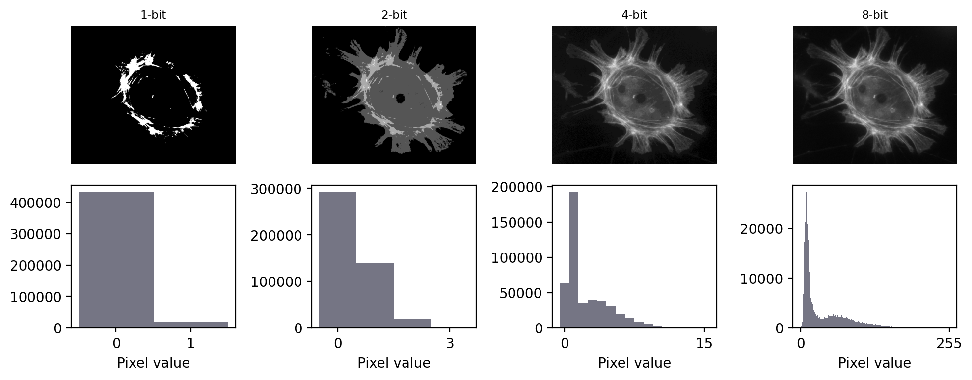
Fig. 21 Representing an image using different bit-depths.

As shown in Fig. 21, a 1-bit image can contain only two values: here, shown as black or white pixels. Such binary images are extremely limited in the information that they can contain, although will turn out to be very useful later when processing images.

A 2-bit image is not much better, containing at most only 4 different values. A 4-bit image can have 16 values. When visualized with a grayscale LUT, this is a substantial improvement. In fact, the eye is not particularly good at distinguishing different shades of gray – making it difficult to see much difference between a 4-bit and 8-bit image. However, the histograms reveal that the 8-bit image contains more fine-grained information.

In practice, computers tend to work with groups of 8 bits, with each group of 8 bits known as a byte. Microscopes that acquire 8-bit images are still reasonably common, and these permit 2⁸ = 256 different pixel values, which fall in the range 0–255. The next step up is a 16-bit image, which can contain 2¹⁶ = 65536 values: a dramatic improvement (0–65535).

Question

What impact would you expect bit-depth to have on the file size of a saved image?

For example, would you expect an 8-bit image to have a larger, smaller or (roughly) equivalent file size to a 16-bit image of the same scene? You can assume the two images have the same number of pixels.

Answer

In general, the file size required to store an image is expected to be higher with a higher bit-depth.

Assuming that the image isn’t compressed, a 16-bit image would require roughly twice as much storage space as a corresponding 8-bit image.

If you have a 1024 x 1024 pixel image that is 8-bit, that should take roughly 1 MB to store. The corresponding 16-bit image would require approximately 2 MB.

Image type

At this point, you might be wondering: what about fractions? Or negative numbers?

In reality, the bit-depth is only part of the story. The type of the image is what determines how the bits are interpreted.

Until now, we have assumed that 8 bits would be used to represent whole numbers in the range 0 – 255, because we have 2⁸ = 256 different combinations of 8 bits. This is an unsigned integer representation.

But suppose we dedicate one of our bits to represent whether the number should be interpreted as positive or negative, with the remaining seven bits providing the magnitude of the number. An image using this approach has the type signed integer. Typically, an 8-bit signed integer can be in the range -128 – 127. Including 0, that still leaves 256 distinct possibilities.

Although the images we acquire are normally composed of unsigned integers, we will later explore the immense benefits of processing operations such as averaging or subtracting pixel values, in which case the resulting pixels may be negative or contain fractional parts. Floating point type images make it possible to store these new, not-necessarily-integer values in an efficient way. That can be important, because we could lose a lot of information if we always had to round pixel values to integers.

Floating point images also allow us to store three special values: \(+\infty\), \(-\infty\) and NaN. The last of these stands for Not a Number, and can represent a missing or impossible value, e.g. the result of 0/0.

Key message

The bit-depth and type of an image determine what pixel values are possible.

How & why points can float

Floating point pixel values have variable precision depending upon whether they are representing very small or very large numbers.

Representing a number in binary using floating point is analogous to writing it out in standard form, i.e. something like 3.14×10⁸, which may be written as 3.14e8. In this case, we have managed to represent 314000000 using only 4 digits: 314 and 8 (the 10 is already baked in to the representation).

In the binary case, the form is more properly something like ± 2^M×N: we have one bit devoted to the sign, a fixed number of additional bits for the exponent M, and the rest to the main number N (called the fraction).

A 32-bit floating point number typically uses 1 bit for the sign, 8 bits for the exponent and 23 bits for the fraction, allowing us to store a very wide range of positive and negative numbers. A 64-bit floating point number uses 1 bit for the sign, 11 bits for the exponent and 52 for the fraction, thereby allowing both an even wider range and greater precision. But again these require more storage space than 8- and 16-bit images.

Common image types & bit-depths

Lots of permutations of bit-depth and type are possible, but in practice three are most common for images:

• 8-bit unsigned integer

• 16-bit unsigned integer

• 32-bit floating point

The representations above are sufficiently ubiquitous that the type is often assumed. Unless otherwise specified, any 8-bit or 16-bit image is most likely to use unsigned integers, while a 32-bit image is probably using floating point pixels.

Conceivably you can have a 32-bit signed/unsigned integer image, or even a 16-bit floating point image, but these are less common in the wild.

Question

The pixels shown on the right all belong to different images.

In each case, identify what possible type an image could have in order to represent the value of the pixel. There can be more than one possible type for each pixel.

Your type options are:

• Signed integer

• Unsigned integer

• Floating point

Answer

The possible image types, from left to right:

1. Signed integer or floating point

2. Unsigned integer, signed integer or floating point

3. Floating point

Note that ‘floating point’ is an option in all cases: it’s the most flexible representation.

Question

What is the maximum pixel value that can be stored in a 16-bit, unsigned integer image?

Answer

The maximum value that can be stored in a 16-bit, unsigned integer image is 2¹⁶-1 = 65535.

Question

What would be the maximum pixel value that can be stored in a 16-bit, signed integer image?

Answer

The maximum value that can be stored in a 16-bit, signed integer image is 2¹⁵-1 = 32767 (since one of the bits is used for the sign, we have 15 remaining).

An image as a matrix of numbers, or just ones and zeros?

You may recall how Fig. 3 showed an image as being a matrix of numbers. That is already a slightly high level abstraction of how the image is actually represented. It’s more accurate to see the image (or, indeed, any digital data) as simply being a long stream of ones and zeros, such as

‘00011001000111110010111100111101001000000010000000011010001000000010001100101110001001000010100000101010010010000011001000011000001001000100001000111011001010110001111000100110000111010100000100110100000111100011001000100100001111000010101000110001001000010010001001001110010000110001011100100011001101000011001100110111001010100011111001010011001011110010100000110000001010100011111100111010010010100100011001010000001111010101111101011101011011000101010110010100101011011110110000111110010001110100111000101101…’

More information is needed about how the pixel values of the image are encoded to interpret these ones and zeros. This includes how should the ones and zeros be split up to represent different values (e.g. in chunks of 8, 16, or some other number?).

The bit-depth is what tells us how big the chunks are, and the type tells us how to convert each chunk into a decimal number.

When bits go bad

We’re now ready to discuss why you absolutely do need to know the basics of bit-depths and image types when working with scientific images.

The main point of Images & pixels is that we need to keep control of our pixel values so that our final analysis is justifiable. There are two main bit-related things that can go wrong when trying to store a pixel value in an image:

1. Clipping: We try to store a number outside the range supported, so that the closest valid value is stored instead. For example, if we try to store -10 in an 8-bit unsigned integer image then the closest value we can actually store is 0. Similarly, if we try to store 500 then the closest valid value is 255.

2. Rounding: We try to store a number that cannot be represented exactly, and so it must be rounded to the closest possible value. For example, if we want to store 6.4 in an 8-bit unsigned integer image then this is not possible; rather, we would need to store 6 instead.

Data clipping

Of the two problems, clipping is usually the more serious, as shown in Fig. 22. A clipped image contains pixels with values equal to the maximum or minimum supported by that bit-depth, and it’s no longer possible to tell what values those pixels should have. The information is irretrievably lost.

Clipping often occurs whenever an image is converted to have a lower bit-depth. During this conversion, not all the original pixel values may be preserved – in which case they must be somehow transformed into the range permitted by the output bit-depth.

This transformation could simply involve clipping the unsupported values (usually very bad), or it could involve rescaling the pixel values first (usually less bad).

Show code cell source Hide code cell source

fig =  create_figure(figsize=(10, 10))

im = load_image('sunny_cell.tif')

# Define the maximum in the 16-bit image (so that it more clearly illustrates the concepts we want to show...)
# (Reader, please ignore this!)
max_value = 800
min_value = 32
im = im.astype(np.float32)
im = im - im.min()
im = im / im.max()
im = im * (max_value - min_value) + min_value
im = im.astype(np.uint16)

# Define colormap & display range
cmap = 'magma'
row = im.shape[0]//2
# vmax = np.percentile(im, 99)
vmax = im.max()
hist_params = dict(bins=100)
line_params = dict(y=row, color=(1, 1, 1), dashes=(4, 2))

# Original image
show_image(im, vmin=0, vmax=vmax, cmap=cmap, title="16-bit original", pos=431)
plt.axhline(**line_params)
show_image(im, vmin=0, vmax=im.max(), cmap=cmap, pos=434)
plt.axhline(**line_params)

plt.subplot(4, 3, 7)
prof_rescaled = im[row, :]
plt.plot(prof_rescaled)
plt.xlabel('x location')
plt.ylabel('Value')
plt.ylim(0, max_value)

show_histogram(im, **hist_params, pos=(4,3,10))

# Clipped to 255
im_clipped = np.clip(im, 0, 255)
show_image(im_clipped, vmin=0, vmax=vmax, cmap=cmap, title="8-bit clipped", pos=432)
plt.axhline(**line_params)
show_image(im_clipped, vmin=0, vmax=im_clipped.max(), cmap=cmap, pos=435)
plt.axhline(**line_params)

plt.subplot(4, 3, 8)
prof_rescaled = im_clipped[row, :]
plt.plot(prof_rescaled)
plt.xlabel('x location')
plt.ylabel('Value')
plt.ylim(0, max_value)

show_histogram(im_clipped, **hist_params, pos=(4,3,11))

# Rescaled, then clipped to 255
im_rescaled = np.clip(im*(255.0/im.max()), 0, 255)
show_image(im_rescaled, vmin=0, vmax=vmax, cmap=cmap, title="8-bit scaled", pos=433)
plt.axhline(**line_params)
show_image(im_rescaled, vmin=0, vmax=im_rescaled.max(), cmap=cmap, pos=436)
plt.axhline(**line_params)

plt.subplot(4, 3, 9)
prof_rescaled = im_rescaled[row, :]
plt.plot(prof_rescaled)
plt.xlabel('x location')
plt.ylabel('Value')
plt.ylim(0, max_value)

show_histogram(im_rescaled, **hist_params, pos=(4,3,12))

plt.tight_layout()

glue_fig("clipping_fig", fig)

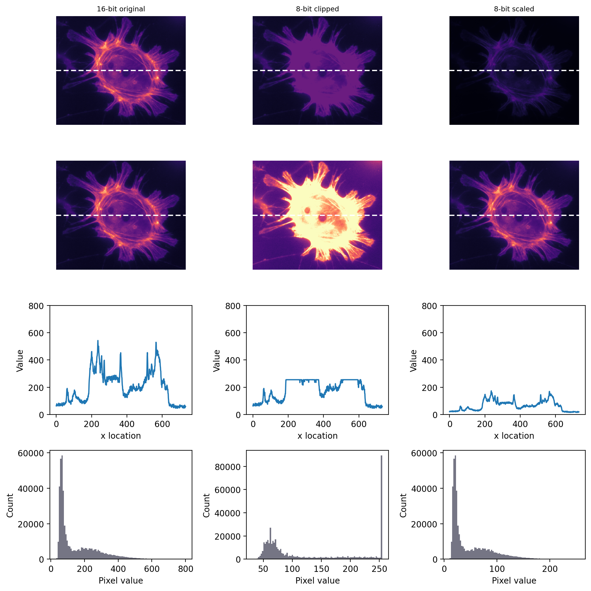
Fig. 22 Storing an image using a lower bit-depth, either by clipping or by scaling the values. The top row shows all images with the same minimum and maximum values to determine the contrast, while the second row shows shows the same images with the maximum set to the highest pixel value actually present (the images are the same, only the LUTs are different). The bottom rows show both a plot of the pixel values through the center of each image and histograms of all the image pixel values. One may infer that information has been lost in both of the 8-bit images, but more much horrifically when clipping was applied. Scaling squeezes the data into a narrow range, which might result in some rounding errors – but most of the information remains intact, with the shapes of the profile plot and histogram remaining similar.

Clipping of high pixel values during acquisition is also called saturation.

However, it’s important to know that clipping can already occur during image acquisition. In fluorescence microscopy, this depends upon three main factors:

1. The amount of light being emitted. Because pixel values depend upon how much light is detected, a sample emitting very little light is less likely to require the ability to store very large values. Although it still might because of…

2. The gain of the microscope. Quantifying very tiny amounts of light accurately has practical difficulties. A microscope’s gain effectively amplifies the amount of detected light to help overcome this before turning it into a pixel value (see Microscopes & detectors). However, if the gain is too high, even a small number of detected photons could end up being over-amplified until clipping occurs.

3. The offset of the microscope. This effectively acts as a constant being added to every pixel. If this is too high, or even negative, it can also push the pixels outside the permissible range.

Avoid clipping your data!

If clipping occurs, we no longer know what is happening in the brightest or darkest parts of the image – which can thwart any later analysis. Therefore during image acquisition, any available controls should be adjusted to make sure clipping is avoided.

Question

When acquiring an 8-bit unsigned integer image, is it fair to say your data is fine so long as your minimum pixel value is 0 and your maximum value is 255?

Answer

No! At least, not really.

You cannot store pixels outside the range 0–255. If your image contains pixels with either of those extreme values, you cannot be certain whether or not clipping has occurred. Therefore, you should ensure images you acquire do not contain any pixels with the most extreme values permitted by the image bit-depth. To be confident your 8-bit data is not clipped, the maximum range would be 1–254.

Question

The bit-depth of an image is probably some multiple of 8, but the bit-depth that a detector (e.g. CCD) can support might not be.

For example, what is the maximum value in a 16-bit image that was acquired using a camera with a 12-bit output?

And what is the maximum value in a 8-bit image acquired using a camera with a 14-bit output?

Assume unsigned integers are used in both cases.

Answer

The maximum value of a 16-bit image obtained using a 12-bit camera is 4095 (i.e. 2¹²-1).

The maximum value of an 8-bit image obtained using a 14-bit camera is 255 – the extra bits of the camera do not change this. But if the image was saved in 16-bit instead, the maximum value would be 16383.

So be aware that the actual range of possible values depends upon the acquisition equipment as well as the bit-depth of the image itself. The lower bit-depth will dominate.

Rounding errors

Rounding is a more subtle problem than clipping. Again it is relevant as early as acquisition.

For example, suppose you are acquiring an image in which there really are 1000 distinct and quantifiable levels of light being emitted from different parts of a sample. These could not possibly be given different pixel values within an 8-bit image, but could normally be fit into a 16-bit or 32-bit image with lots of room to spare. If our image is 8-bit, and we want to avoid clipping, then we would need to scale the original photon counts down first – resulting in pixels with different photon counts being rounded to have the same values, and their original differences being lost.

Nevertheless, rounding errors during acquisition are usually small: it may not really matter if we can’t tell the difference between detecting 1,000 photons and 1,003 photons.

Rounding can be a bigger problem when it comes to processing operations like filtering, which often involve computing averages over many pixels (see Filters). The good news is that at this post-acquisition stage we can convert our data to floating point and then get fractions if we need them.

Floating point rounding errors

As a full disclosure, I should admit that using floating point types is only a partial solution to rounding issues. Even a 64-bit floating point image cannot store all useful pixel values with perfect precision, and seemingly straightforward numbers like 0.1 are only imprecisely represented.

But this is not really unexpected: this binary limitation is similar to how we cannot write 1/3 in decimal exactly. We can write 0.3333333 but our level of precision will depend upon our willingness to continue adding 3’s after the decimal point.

In any case, rounding 0.1 to 0.100000001490116119384765625 (a possible floating point representation) is not so bad as rounding it to 0 (an integer representation), and the imprecisions of floating point numbers in image analysis are usually small enough to be disregarded.

See https://xkcd.com/217/ for more information.

More bits are better (usually)

From considering both clipping and rounding, the simple rule of bit-depths emerges: if you want the maximum information and precision in your images, more bits are better. This is depicted in Fig. 23.

When given the option of acquiring a 16-bit or 8-bit image, most of the time you should opt for the former.

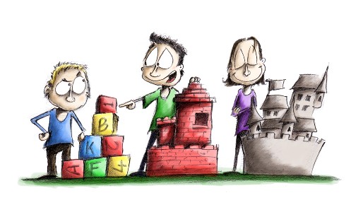
Fig. 23 Illustration of the comparative accuracy of (left to right) 8-bit, 16-bit and 32-bit images. If an 8-bit image is like creating a sculpture out of large building blocks, a 16-bit image is more like using Lego and a 32-bit floating point image resembles using clay. Anything that can be created with the blocks can also be made from the Lego; anything made from the Lego can also be made from the clay. This does not work in reverse: some complex creations can only be represented properly by clay, and building blocks permit only a crude approximation at best. On the other hand, if you only need something blocky, it’s not really worth the extra effort of Lego or clay. And, from a very great distance, it might be hard to tell the difference.

Question

Although more bits are better is a simple rule of thumb we can share with those who do not know the subtleties of bit-depths, it should not be held completely rigorously.

Can you think of any circumstances when more bits might not be better?

Answer

Reasons why a lower bit depth is sometimes preferable to a higher one include:

• A higher bit-depth leads to larger file sizes, and potentially slower processing. For very large datasets, this might be a bigger issue that any loss of precision found in using fewer bits.

• The amount of light detected per pixel might be so low that thousands of possible values are not required for its accurate storage, and 8-bits (or even fewer) would be enough. For the light-levels in biological fluorescence microscopy, going beyond 16-bits would seldom bring any benefit.

But with smallish datasets for which processing and storage costs are not a problem, it is safest to err on the side of more bits than we strictly need.