Python: Measurements & histograms

Here, we will explore how to make measurements and generate histograms with Python.

# Our usual default imports
import sys
sys.path.append('../../../')

from helpers import *
import matplotlib.pyplot as plt

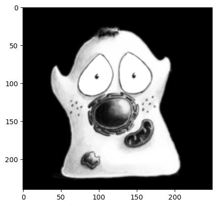
# Read an image - we need to know the full path to wherever it is
im = load_image('happy_cell.tif')

# Show the image
plt.imshow(im, cmap='gray')
plt.show()

Introduction to NumPy arrays

The images we are working with in Python are NumPy arrays - https://numpy.org

Rather than plotting the image with plt.imshow, we can also simply print its values. Since there can be a lot of values (i.e. millions of pixels per image), only a few are shown by default.

print(im)

[[2. 2. 2. ... 2. 2. 2.]
 [2. 2. 2. ... 2. 2. 2.]
 [2. 2. 2. ... 2. 2. 2.]
 ...
 [2. 2. 2. ... 2. 2. 2.]
 [2. 2. 2. ... 2. 2. 2.]
 [2. 2. 2. ... 2. 2. 2.]]

If we want to know how many values are in an image, we can query its shape.

This returns the size in the order (height, width).

print(im.shape)

(240, 250)

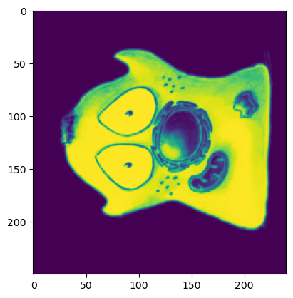
Whenever we have a 2D NumPy array, we can easily transpose it - which will switch the width and height values.

im2 = im.transpose()
print(im2.shape)
plt.imshow(im2)
plt.show()

(250, 240)

Calculating statistics

A more meaningful benefit of working with NumPy arrays, for our purposes at least, is that they enable us to calculate some summary statistics extremely easily.

For example, to compute the average (mean) pixel value we can simply use im.mean().

im.mean()

23.031446

If that’s the last thing we add to a code cell, then the result will be displayed in our notebook.

However, if we want to print multiple values - and multiple statistics - in quick succession we should use the print function again.

print(im.mean())
print(im.min())
print(im.max())
print(im.std())

23.031446
2.0
65.75
27.156355

Formatting output

Things become more readable if we add some extra text, rather than just printing numbers.

One of the easiest ways to do this is to use an ‘f-string’, which is in the form f'Some text {some_variable}.

The part between the braces {} can be a calculation, and if you add :.2f at the end this will optionally limit the number of decimal places (here, to two).

print(f'Mean:     {im.mean()}')
print(f'Minimum:  {im.min():.1f}')
print(f'Maximum:  {im.max():.2f}')
print(f'Std.dev.: {im.std():.3f}')

Mean:     23.03144645690918
Minimum:  2.0
Maximum:  65.75
Std.dev.: 27.156

Generating histograms

We can now try to generate image histograms, using plt.hist.

You might expect plt.hist(im) to work, just as plt.imshow(im) did previously. However, the result can be a bit surprising.

plt.hist(im)
plt.show()

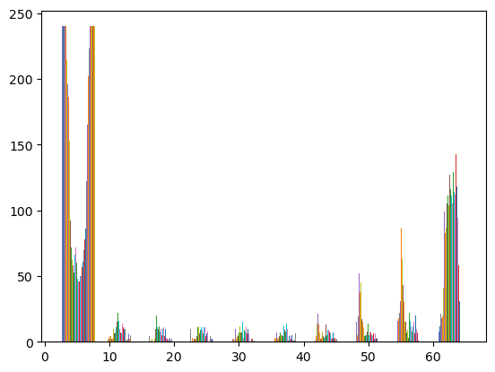
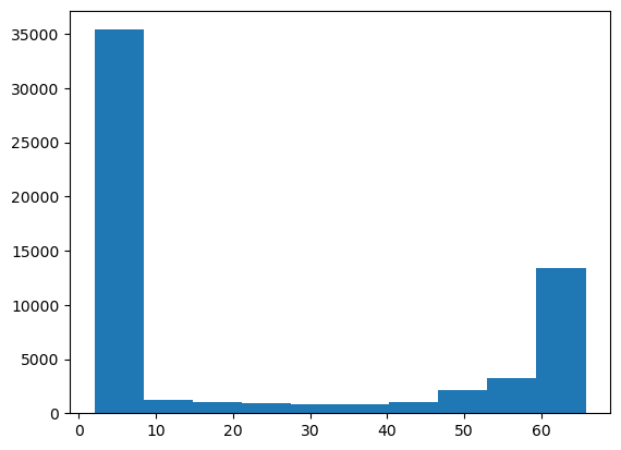
The problem is that the image is 2D, and plt.hist is expecting just a single 1D list of values. We can generate that with a call to .flatten(), and use the flattened array to create the histogram.

print(f'Shape before flatten(): {im.shape}')
im_flat = im.flatten()
print(f'Shape after flatten(): {im_flat.shape}')

Shape before flatten(): (240, 250)
Shape after flatten(): (60000,)

plt.hist(im_flat)
plt.show()

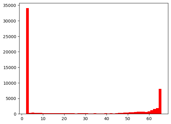
As with plt.imshow, we have lots of options to customize the histogram. This includes the ability to set the color or number of histogram bins.

plt.hist(im.flatten(), bins=50, color='red')
plt.show()

Parentheses

It may initially be confusing why we sometimes need parentheses () and sometimes we don’t, e.g. im.flatten() vs. im.shape.

As a general rule, parentheses indicate that we’re calling a method that does something (e.g. prints a value, calculates an average, flattens an array).

When we don’t see parentheses, this indicates that we’re accessing a field or property (e.g. the shape of an array).

In practice, the distinction can sometimes be a bit murky as you get deeper into Python - but it helps as a general guide.